Marc Lata

MEGR 8172

12/12/2018

Take Home Final

The goal if this take-home final is to numerically solve the time evolution of a double pendulum system using a forward Euler method. The double pendulum has the following structure:

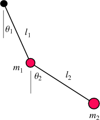
Figure 1: Double Pendulum

The governing equations of this system is given as:

a)

The first step to solve this system is to write this system in the form

To do this I will introduce the angular velocity as a variable such that:

And my vectors will be:

Now, in order to write the governing equations in terms of these vectors, let me in substitute , and :

Now, I must solve these for , and . To do this, I will utilize Matlab’s symbolic solving functionality. I developed the following script to solve this system (solvesystem.m):

%Solve double pendulum system

syms m1 m2 l1 l2 g theta1 theta2 omega1 omega2 alpha1 alpha2

eqn1 = (m1 + m2)*l1^2 * alpha1 + m2*l1*l2*alpha2*cos(theta1-theta2) + m2*l1*l2*omega2^2*sin(theta1-theta2) + g*l1*(m1+m2)*sin(theta1) == 0;

eqn2 = l2*alpha2 + l1*alpha1*cos(theta1-theta2) - l1*omega1^2*sin(theta1-theta2) + g*sin(theta2) == 0;

[x1,x2] = solve(eqn1,eqn2,alpha1,alpha2)

This gives me the following results:

x1 =

-(l1*m2*cos(theta1 - theta2)*sin(theta1 - theta2)*omega1^2 + l2*m2*sin(theta1 - theta2)*omega2^2 + g*m1*sin(theta1) + g*m2*sin(theta1) - g*m2*cos(theta1 - theta2)*sin(theta2))/(l1*(m1 + m2 - m2*cos(theta1 - theta2)^2))

x2 =

(l1*m1*omega1^2*sin(theta1 - theta2) - g*m2*sin(theta2) - g*m1*sin(theta2) + l1*m2*omega1^2*sin(theta1 - theta2) + g*m1*cos(theta1 - theta2)*sin(theta1) + g*m2*cos(theta1 - theta2)*sin(theta1) + l2*m2*omega2^2*cos(theta1 - theta2)*sin(theta1 - theta2))/(l2*(m1 + m2 - m2*cos(theta1 - theta2)^2))

Now I can tell Matlab how to take the derivative of my vector (xdot.m):

%Derivative of x vector

function q = xdot(x,m1,m2,l1,l2,g)

theta1 = x(1);

theta2 = x(2);

omega1 = x(3);

omega2 = x(4);

alpha1 = -(l1*m2*cos(theta1 - theta2)*sin(theta1 - theta2)*omega1^2 + l2*m2*sin(theta1 - theta2)*omega2^2 + g*m1*sin(theta1) + g*m2*sin(theta1) - g*m2*cos(theta1 - theta2)*sin(theta2))/(l1*(m1 + m2 - m2*cos(theta1 - theta2)^2));

alpha2 = (l1*m1*omega1^2*sin(theta1 - theta2) - g*m2*sin(theta2) - g*m1*sin(theta2) + l1*m2*omega1^2*sin(theta1 - theta2) + g*m1*cos(theta1 - theta2)*sin(theta1) + g*m2*cos(theta1 - theta2)*sin(theta1) + l2*m2*omega2^2*cos(theta1 - theta2)*sin(theta1 - theta2))/(l2*(m1 + m2 - m2*cos(theta1 - theta2)^2));

q = [omega1;omega2;alpha1;alpha2];

The Forward Euler method can be written as:

This can be programmed very easily as (forwardeuler.m):

%Forward Euler Function(

function q = forwardeuler(x,dt,m1,m2,l1,l2,g)

xd = xdot(x,m1,m2,l1,l2,g);

q = x + xd*dt;

Now, I can implement this forward Euler method for the initial conditions provided(driver.m):

%Initial Conditions

x(:,1)= [.8*a; 1.1*a; 0; 0];

for i = 2:nt+1

x(:,i) = forwardeuler(x(:,i-1),dt,m1,m2,l1,l2,g);

[K(i),V(i)] = energy(x(:,i), m1, m2, l1, l2, g);

E(i) = K(i) + V(i);

end

I have also implemented in this step the energy calculation (energy.m):

%Energy Calculation

function [K,V] = energy(x, m1, m2, l1, l2, g)

th1 = x(1);

th2 = x(2);

w1 = x(3);

w2 = x(4);

K = (1/2)*m1*l1^2*w1^2 + (1/2)*m2*l1^2*w1^2 + (1/2)*m2*l2^2*w2^2 + m2*w1*l1*w2*l2*cos(th1-th2);

V = -(m1+m2)*g*l1*cos(th1) - m2*l2*g*cos(th2);

For the following physical parameters and time step (main.m);

%System Parameters

a = strlength("Lata")/5; %Name Dependent Parameter

m1 = 2; %Kg

m2 = 1.5; %Kg

l1 = 1.1 * a; %Meters

l2 = 1.8 * a; %Meters

g = 9.81; %m/s^2

T = 25; %Seconds

dt = 1e-2; %Seconds

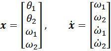
I get the following results:

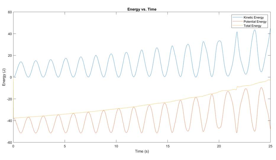
Figure 2: Double Pendulum Simulation with dt =.01

You can see that the energy in my system is constantly increasing, and there is no regularity to the oscillations. If I decrease my time step to 1e-5, I can get results that appear to be more representative of the real physical system:

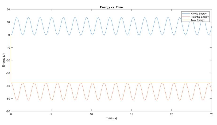
Figure 3: Double Pendulum Simulation with dt = 1e-5

In this simulation, my energy remains constant, and the pendulums appear to be in some fixed oscillatory path.